Bad Science: Converting TLEs to Keplerian Elements
Don't Do This
Converting TLEs To Keplerian Coordinates with Simple Math
NORAD (North American Aerospace Defense Command) tracks most decently sized objects in space, and uses the SGP4 model to characterize the orbits of these objects. The traditional format for this data is the "Two Line Element Set," or TLE for short, and you can access these TLEs at space-track.org.
In theory, TLEs will help you characterize the orbit of a satellite, which in turn allows you communication with the satellite, orbital maneuvers, or remote sensing. Of course, to do this you'll need to know how to engage with the data.
The correct method of using the data is by employing the official SGP4 Propagation Library (Note: This is EAR controlled software). That isn't as fun as doing it ourselves, so lets run over the math.
Warning: You shouldn't do this
Two line element sets were created using NORAD's radar tracking system, in house software, and a certain degree of estimation. This process isn't totally transparent to us, so we cannot account for error correctly. If real money rides on this, use the SGP4 Propagation Library mentioned above. I will detail how to do that in a different blog post.
Dr. T. S. Kelso of Celestrak fame put it best:
The elements in the two-line element sets are mean elements calculated to fit a set of observations using a specific model—the SGP4/SDP4 orbital model. Just as you shouldn't expect the arithmetic and geometric means of a set of data to have the same value, you shouldn't expect mean elements from different element sets—calculated using different orbital models—to have the same value. The short answer is that you cannot simply reformat the data unless you are willing to accept predictions with unpredictable errors.
Obtain TLEs
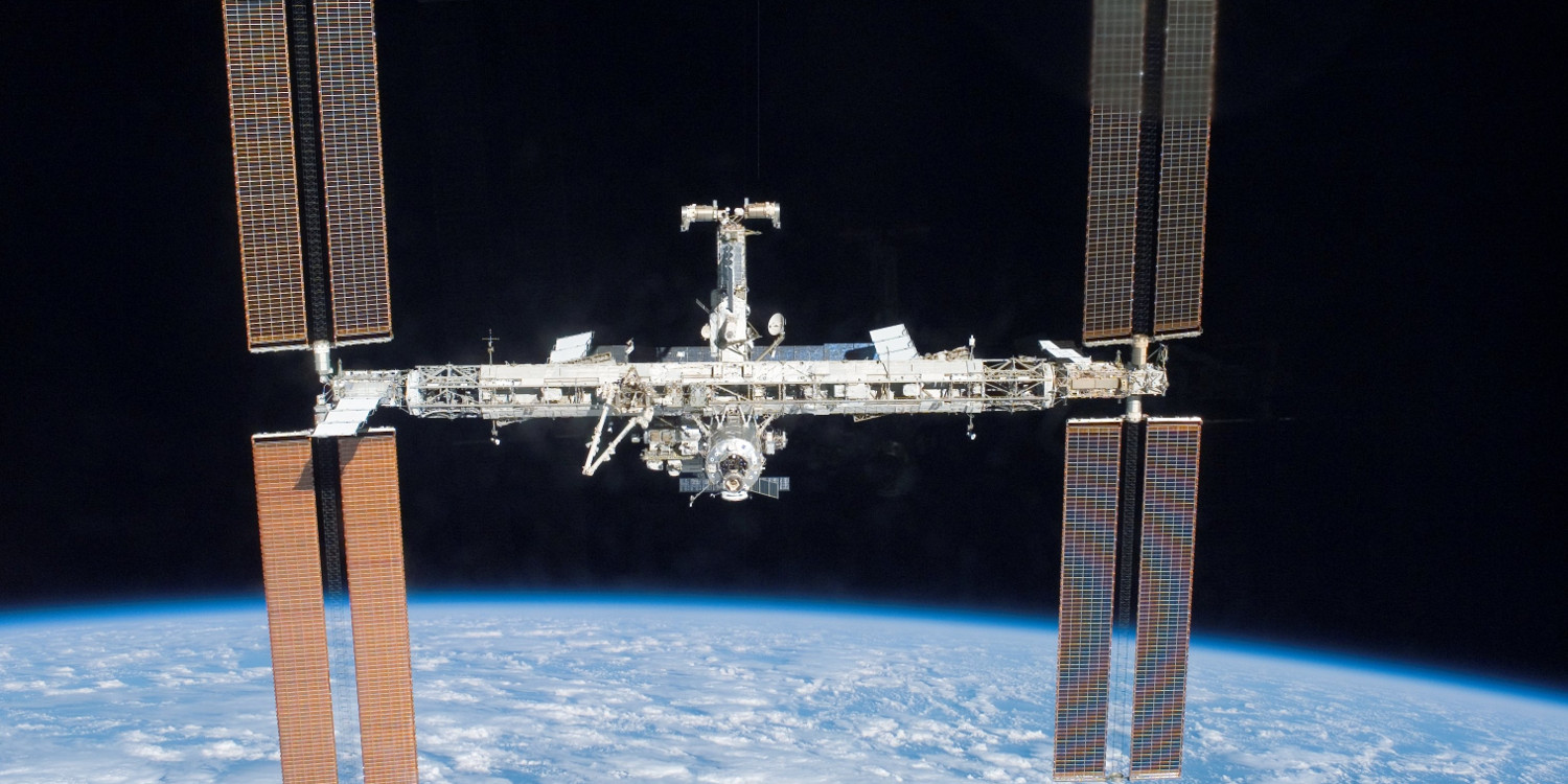
You can obtain TLEs from Celestrak and space-track.org. I chose to grab some TLEs for the ISS and some Microsat-R debris using the celestrak satellites page. Microsat-R was an Indian satellite used as target practice for an anti-satellite weapon. India tried to mitigate the space debris risk by hitting a low altitude target, but NASA Administrator Jim Bridenstine pointed out that, due to the solar minimum, this debris will take longer than normal to decay. Worse, the explosive force propelled 24 pieces into orbits with apogees above the 400 km altitude of the ISS. While the thought of a debris strike on the ISS is chilling, it does provide an excellent educational opportunity for students taking orbital mechanics.
MICROSAT-R
1 43947U 19006A   19178.81152645  .00159043  20002-5  69067-4 0  9994
2 43947  96.6118  92.0822 0043792 270.1611  89.4676 16.20059674 24697

ISS (ZARYA)
1 25544U 98067A   19178.82735530  .00002515  00000-0  49918-4 0  9997
2 25544  51.6428 308.4904 0008116  89.4883  70.1063 15.51247238176900
Historical Note: The ISS is sometimes referred to as Zarya because that is the name of the first module to be placed into orbit.
Using this key, we can extract the six Keplerian ephemerides from each.
| element                   | ISS         | Microsat-R  |
|---------------------------|-------------|-------------|
| inclination (deg)         | 51.6428     | 96.6118     |
| RAAN (deg)                | 308.4904    | 92.0822     |
| eccentricity              | .0008116    | .0043792    |
| argument of perigee (deg) | 89.4883     | 270.1611    |
| mean anomaly (deg)        | 70.1063     | 89.4676     |
| mean motion (rev/day)     | 15.51247238 | 16.20059674 |
Keplerian Elements
The traditional Keplerian element set are six numbers which fully define the geometry of an orbit. This solution is largely useless without an additional time component, which TLEs represent as an Epoch.
- eccentricity, \(e\)
- semimajor axis, \(a\)
- inclination, \(i\)
- Longitude of the ascending node, \(\Omega\)
- argument of of periapsis, \(\omega\)
- true anomaly, \(\nu\)
- Epoch, \(t\)

By Lasunncty at the English Wikipedia, CC BY-SA 3.0, link
Four of the six elements provided in the TLE do not match the traditional Keplerian orbital elements. I'll go over why when I explore SGP4. For now, use the following steps to convert to traditional Keplerian elements.
Longitude of the Ascending Node From TLE
In the case of Earth orbits, longitude of the ascending node and right ascension of the ascending node happen to be equal. All we have to do is convert to radians.
$$\Omega = RAAN \frac{\pi}{180^\circ}$$
Argument of Periapsis
Argument of periapsis and argument of perigee are synonyms. Once we convert to radians, were all set.
$$\omega = \omega^* \frac{\pi}{180^\circ}$$
Semimajor Axis
Semimajor axis is computed from mean motion. First, we must convert the mean motion provided (\(n^*\)) into a mean motion expressed in radians per second (\(n\)).
$$n = n^* \times \frac{1 day}{86,400 s} \times \frac{2\pi \, radians}{revolution}$$
Next, we compute the period of the orbit.
$$T = n \times 2\pi$$
Finally, we directly compute semi-major axis from the orbital period. A commonly used equation for orbital period is:
$$\frac{a^3}{T^2} = \frac{\mu}{4\pi^2}$$
\(\mu\) is the gravitational parameter of Earth, \(3.986004418 \times 10^{14} m^3 s^{-2}\)
Solving...
$$a = \sqrt[3]{\frac{T^2\mu}{4\pi^2}}$$
True Anomaly From TLE
First, convert mean anomaly to radians.
$$ M = M^* \times \frac{\pi}{180 ^\circ} $$
Second, obtain eccentric anomaly using Kepler's equation. It can't be solved using traditional algebra, but the Newton Rhapson algorithm will converge rapidly.
Kepler's Equation: \(M = E-e \times \sin(E)\)
Newton Rhapson Setup: \(E_{k+1} = M + e \sin(E_{k})\), \(E_{1} = M\)
Solve the above equation until convergence is reached. A quick and easy way to approximate convergence is to evaluate whether \(E_{k+1}\) is less than 1% different than \(E_{k}\).
$$\left\|\frac{E_{k+1} - E_{k}}{E_{k+1}}\right\| < 0.01$$
Pro Tip: You can set up Newton Rhapson's algorithm on most calculators such that the equation iterates every time you hit the "enter" key. On a TI-89, type \(\pi\), enter, then type out
M* + e*sin(ans), and mash enter repeatedly until the result stops changing. Practice this before your next test!
Once Eccentric anomaly is known, you can directly compute true anomaly with the following equation, which comes from the geometry of an ellipse.
$$\cos(\nu) = \frac{\cos(E) - e}{1-e\cos(E)}$$
$$\nu = \arccos \bigg( \frac{\cos(E) - e}{1 - e\cos(E)} \bigg)$$
Next Steps
Now that the full Keplerian elements are known, you may be tempted to calculate the distance between the Microsat-R debris and the ISS, but the TLEs we collected are not temporally co-located (they weren't collected at the same time). The very next step would be to propagate the older TLE so that it has the same time as the newer TLE. Next, you would propagate both for a couple of revs, making note of the distance between the objects at each point in time.
All of this propagating will cause the difference between your solution and the true orbit to would grow rapidly. The problem is that we need to account for atmospheric drag and gravitational effects (such as J2).
This is fundamentally why NORAD uses SGP-4. You'll notice that the TLE is packed with information that describes the perturbing effects on the orbit. For example, the \(B^*\) ("B-Star") term describes the atmospheric drag experienced by the satellite, and the first and second time derivatives of mean motion describe the evolution of the satellite orbit over time.
For a school assignment, this process is good for building intuition and understanding the orbital mechanics. However, if you need accurate results, you should utilize the space-track API to constantly update your TLEs, and you should use the official SGP-4 propagation package to determine coordinates in other systems.
Bibliography
- Celestrak Report No 3
- Celestrak
- space-track.org
- Bate, Mueller, and White, "Fundamentals of Astrodynamics," Copyright 1971